CT Concepts
1. Introduction
This first chapter is a brief overview of the main concepts we come across in CT. While everything discussed here is essential knowledge for CT scanning, don't worry if you don't totally grasp all of the concepts straight away. We will be readdressing all of these later in the course when we discuss how we change scanning and post processing factors to influence image quality and dose.
2. X, Y and Z Axis
Because we are acquiring a 3-dimensional volume in CT, we need to be able to explain which direction (or axis) the image is being viewed and acquired. Imagine you are standing in front of the CT scanner, looking down the table and through the other side of the gantry:
X-axis - is in the horizontal plane, parallel to the floor, left to right
Y-axis - is in the vertical plane, perpendicular to the floor, top to bottom
Z-axis - is also parallel to the floor, but is along the length of the table, in and out of the gantry

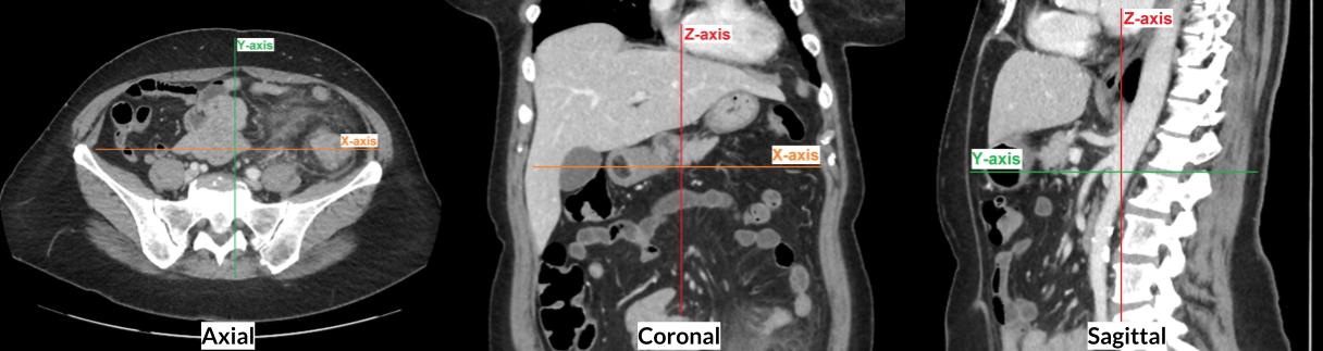
If we were to look at the images of a CT Abdomen where the patient was positioned supine feet first, the coordinates would be as follows:

3a. Slice Thickness
Slice thickness can be broken into two categories:
Detector Slice Thickness: This is the z-axis thickness of each individual detector slice within the detector array. The smaller the slice thickness, the better the spatial resolution of the images. Most modern scanners have a slice thickness <1mm. This is discussed in more detail on the next page.
Reconstructed Slice Thickness: This is the depth of the voxels on a multiplanar reconstructed image. The operator can select any thickness equal to or higher than the detector slice thickness. Each slice makes up an image. The slices are then stacked together to form a series of images which the viewer can scroll through. An analogy for this is cutting a loaf of bread into slices of a certain thickness, then stacking them back together in a loaf and viewing each slice of bread one by one. There are both pros and cons relating to slices of different thicknesses, which will be discussed in the next module.
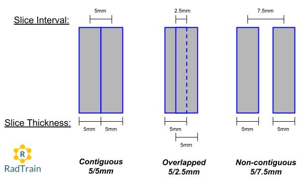
3b. Slice Interval
This is the distance between the centre of two adjacent slices within a series of images.
For a contiguous image, the slice interval will match the slice thickness, so the next slice will start where the previous slice ends.
If the slice interval is less than the slice thickness, then this will result in overlapped slices. This will create more images in the series.
If the slice interval is more than the slice thickness, then this will result in non-contiguous slices (gaps between the slices). This will create less images in the series, however the anatomy that falls within the gap will not be visible.
The majority of multiplanar reconstructions used in CT are contiguous, because it is the optimal balance between not having too many images (as we get with overlapped slices) and not leaving any anatomy out of the images (as we get with non-contiguous slices).
Overlapped slices can be useful in some instances, especially when viewing very small and intricate anatomy such as small blood vessels on an angiogram. Non-contiguous slices run the risk of missing anatomy and pathology, so they are rarely used (except when scanning HRCT lungs as a dose reduction techinque - more on this later).
The video below demonstrates what the above three examples of contiguous, overlapped and non-contiguous reconstructions would look like on a Chest CT. Try to pick a single bronchial branch and follow it through the series to give you an idea of how the different interval settings affect the images:

4. Detector Size and Slice Number
Think of a detector as an array of individual cells, stuck together to form a lattice along the X- and Z-axis. Each cell sends a signal to the processor when it is excited by a photon. This signal is then processed to form a pixel within the image (this isn't exactly how it works, but it is easiest to think of it this way when discussing slice thickness).
The detector size indicates the maximum possible z-axis coverage per rotation, which determines how quickly a scan can be taken. The larger the detector coverage, the more coverage per rotation and therefore the quicker the scan.
In the early days of axial scanning, the number of slices in a detector and the size of those slices would directly correlate to the detector size using the following formula:
Detector Size= Number of Slices x Slice Thickness
Example: 20mm detector = 4 slices x 5mm thickness

Today, this formula is not so straight forward. Many vendors use slice number as a marketing tool, and it does not accurately represent the z-axis coverage capable of the scanner.
For example, a 64 slice and 128 slice scanner can both have a 40mm z-axis detector size. How? The 128 slice scanner has a software that creates a 50% overlap on their axial scans, and therefore the ability to virtually reconstruct 128 slices at 0.312mm thickness (128x0.312 = 40mm). In this example, both scanners have the same scan speed because they have the same z-axis detector size.
So don't be fooled by slice number, the real determiner for scan speed is the detector size. Modern multidetector CT scanners have detector size ranging from 20mm to 160mm, so there is quite a lot of variation in scan speed options.
5. Beam Collimation
This value determines the z-axis coverage per rotation, which is controlled by the pre-patient collimators.
The maximum beam width is equal to the detector size, but most scanners allow the operator to select a narrower beam width (i.e. not use all of the detector slices). A narrower beam width will result in sharper images, but longer scan times.

The diagram above shows two different beam collimation settings: (Left) Wide 40 mm, which uses the entire detector size on a scanner with a 40 mm detector; (Right) Narrow 20 mm, which only uses the middle half of a 40 mm detector.
6. Raw Data vs Thin Slice Series
Have you ever been asked by the radiologist to send the "raw data" of a scan to PACS? Well now is your chance to get on your high-horse and (very politely) correct them.
Raw Data is commonly confused with the Thin Slice series, but they are two separate things.
Raw Data is the series of electrical signals sent by the detectors to the image processor. It contains all the necessary information required to generate a digital image. You cannot view raw data as an image, nor can you send it to PACS as a series.
A Thin slice series is reconstructed from the raw data, which is then used to view and post-process images of varying slice thickness and orientation (called multiplanar reconstructions). The slice thickness of thin slice data is equal to the slice thickness of the detector slices (which is the thinnest possible slice thickness).
7. Hounsfield Unit (CT Number)
Hounsfield Unit (HU) is a value assigned to each pixel in the raw data that determines the level of brightness in the reconstructed image. It is calculated by the amount of attenuation recorded, relative to water (which is given a value of zero). Any pixel above zero will appear brighter than water, and any pixel below zero will appear darker.
Factors that affect attenuation include beam energy (kVp) and the atomic number (or density) of the anatomical structure. This will be discussed in depth later on.
On the Hounsfield scale:
Water = 0 (gray)
Bone > +1000 (white)
Air < -1000 (black)
Fat = -110 to 0
Grey Matter = 20
White Matter = 35
Unenhanced Vessel = 10 to 100
Muscle / Unenhanced Liver = 30 to 150
8. Window Width/Level
These settings determine which HU are displayed on the image viewer. They do not manipulate the assigned HU of each pixel, as this is embedded in the raw data.
Window Width - is the range of HU values, and determines the contrast
Window Level - is the HU in the centre of the range (width), and determines the brightness
The example below shows a Window Width of 2000 and a Window Level of 500. This means the HU being displayed range from -500 to +1500.

The table below provides some standard WW/WL settings for viewing different anatomical structures:

9. Multiplanar Reconstructions
A series of images can be reconstructed in any angle and slice thickness that the operator desires. The three orthogonal reconstruction planes are:
Axial - along the z-axis, looking from the patient’s toes to head
Coronal - along the y-axis, looking from the patient’s front to back
Sagittal - along the x-axis, looking from the patient’s right to left
Oblique reconstructions define any angled plane other than the orthogonal ones.
The operator can also set the slice thickness and slice interval, DFOV, and the reconstruction mode (see below) for each series.
It is best to reconstruct multiplanar images using a thin slice series, as this will produce the best spatial resolution for the coronal, sagittal and oblique series.
10. Reconstruction Mode
The reconstruction mode determines what HU is assigned to each voxel. A voxel includes all the data in the 2D pixel plane, plus the data in the third-dimension determined by the slice thickness. There are three reconstruction modes to display this data:
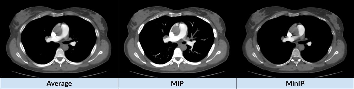
1. Average - this applies an average value to all the individual HU within the voxel. This is the most common reconstruction mode used in multiplanar reconstructions, as it provides the truest representation of the image.
For example, if the voxel spans over 3 pixels with individual HU of 10, 12, and 20, the average HU would be 14
2. MIP (Maximum Intensity Projection) - this uses the highest value from all the individual HU within the voxel. This is commonly used in angiograms or through the lungs to better visualise the smaller vessels or bronchi. You would generally provide both an Average and a MIP of the same multiplanar reconstruction to provide both perspectives.
For example, if the voxel spans over 3 pixels with individual HU of 10, 12, and 20, the MIP HU would be 20
3. MinIP (Minimum Intensity Projection) - this uses the lowest value from all the individual HU within the voxel. The uses for this mode are sporadic and not very common. An example may be to visualise non-calcified plaque within a contrast-enhanced vessel, however this is usually visualised adequately on the Average or MIP images.
For example, if the voxel spans over 3 pixels with individual HU of 10, 12, and 20, the MinIP HU would be 10
The thicker the slice, the larger the range of pixels used to calculate the HU of the voxel. This results in:
Volume averaging for Average mode
Usually brighter images for MIP (because there is more chance of a high HU pixel being included in the range)
Usually darker images for MinIP (because there is more chance of a low HU pixel being included in the range)
11. DFOV and SFOV
Display Field of View (DFOV) is the diameter of a reconstructed image.
Scan Field of View (SFOV) is the diameter of the acquired raw data.
DFOV can be manipulated by the operator in post-processing, given it is within the SFOV.
SFOV is fixed and cannot be changed. If an area of anatomy is outside the SFOV during the scan, it will not be imaged.
12. Reconstruction Algorithm / Kernel
Kernels are settings that are applied to reconstructed data to change the levels of noise and spatial contrast.
Generally there is a scale ranging from smooth (good for soft tissue) to sharp (good for bone).
They are not filters that can be turned on or off the image - if the operator would like an image with different smooth/sharp levels, they need to reconstruct another series from the raw data.